Run/Access Jupyter Notebook From Remote Server

Jupyter Notebooks extend the console-based approach to interactive computing in a qualitatively new direction, providing a web-based application suitable for capturing the whole computation process: developing, documenting, and executing code, as well as communicating the results.

Install Jupyter Notebook on the Server

Connects to the OPH cluster with you user Account

ssh -XY username@remote_ip_address

the remote_ip_address of the OPH cluster is 137.204.50.177, the username is your unibo account

Activate your conda environment (es. my_env)

(base)[username@ophfe2 ~]$ conda activate my_env

If the Jupyter Notebook (or JupyterLab) package is not already installed, add it to your virtual environment by executing the following command:

(my_env)[username@ophfe2 ~]$ conda install jupyter

This command installs Jupyter Notebook and its dependencies within the currently activated (my_env) virtual environment .

Alternatively, if you prefer JupyterLab, you can install it with the following command:

(my_env)[username@ophfe2 ~]$ conda install -c conda-forge jupyterlab

Both Jupyter Notebook and JupyterLab are web-based user interface for Project Jupyter (JupyterLab provides a more integrated and extensible environment for working with Jupyter Notebooks)

Running Jupyter Notebook on the Server

On the OPH Cluster, initiate Jupyter Notebook with the –no-browser option and specify a port using the following command:

(my_env)[username@ophfe2 ~]$ jupyter notebook --no-browser --port=8080 &

When you start a notebook server with token authentication enabled (default), a token is generated to use for authentication. This token is logged to the terminal, so that you can copy/paste the URL into your browser:

[I 18:32:06.663 NotebookApp] Jupyter Notebook 6.5.6 is running at:
[I 18:32:06.663 NotebookApp] http://localhost:8080/?token=5ea93f806c0b49767b38587daced8f685561c4fa9b1333bc

Then, open a new terminal in your local machine and establish an SSH tunnel for port forwarding, like this:

ssh -L 8080:localhost:8080 username@137.204.50.177

8080:localhost:8080 sets up a tunnel from your local machine’s port 8080 to the remote server’s localhost on port 8080 (adjust the port numbers according to your specific requirements). After establishing the SSH connection with the tunnel, you can use this tunnel for accessing services on the remote server as if they were running locally on your machine.

Now you can open a browser and go to http://localhost:8080. It will appear in the Jupyter notebook. You’ll need to write the token (generated when you open jupyter in your remote terminal). You should be able to select your notebook located in your /home directory on the OPH server.

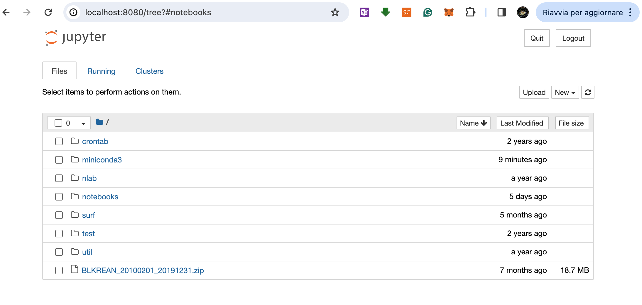
Fig 2. Screenshot of the Jupyter Notebook web-based user interface (your /home directory in the Cluster)

Submit your notebooks on the compute nodes

Let create a simple jupyter notebook called mynotebook.ipynb:

# import libraries
import numpy as np
import matplotlib.pyplot as plt

# Define the grid for the independent variables with the numpy.arange() function
z0, z1, dz = 0., 10., 0.1
z = np.arange(z0, z1, dz)

# Define spectral irradiance as function of depth (is described by decreasing exponential functions)
Qsr = 170   #penetrative Radiative Flux at sea surface in W/m^2
R = 0.58    #fraction of Qsr at lambda > 700 nm
xi0 = 0.35  #extinction length scale at lambda > 700 nm
L = Qsr*R*np.exp(-z/xi0)

# Create a figure and one single window Axes with the pyplot.subplots() function
fig, ax = plt.subplots(figsize=(6,6))

# Plot y versus x as lines in the Axes with the axes.plot() function
ax.plot(L, z)

# Set title and x-y axis labels for the Axes with the axes.set_title() function
ax.set_title('Penetration of Solar Radiation in the Upper Ocean', fontsize=14)
ax.set_xlabel('Flux [W/m2]', fontsize=16)
ax.set_ylabel('Depth [m]', fontsize=16)

# Adds gridlines to the Axes with the axes.grid() function
ax.grid(linestyle='--', color='gray')

# Set the y-axis view limits for the Axes with the axes.set_ylim() function
ax.set_ylim(-1, z1)
ax.set_xlim(0, Qsr)

# Invert the y-axis with the axes.invert_yaxis() function
ax.invert_yaxis()

# Display the figure with the pyplot.show() function
# plt.show()  #fig

# Save the current figure to a file with the pyplot.savefig() function
fig.savefig('plot_line01.png')

Now, create a job submission script (let’s call it jupyter.sh) to run the mynotebook.ipynb on the OPH compute nodes

#!/bin/bash
#SBATCH --job-name=jupyter_notebook
#SBATCH --nodes=1
#SBATCH --ntasks-per-node=1
#SBATCH --mem=8G
#SBATCH --time=00:05:00
#SBATCH --output=output_%j.txt
#SBATCH --error=output_%j.err

# load modules or conda environments here (check if the module is available)
# module load anaconda3/2023.3
source /home/PERSONALE/francesco.trotta4/miniconda3/etc/profile.d/conda.sh

# Activate your specific Conda environment
conda activate my_env

# Run Jupyter (srun {{command}})
srun jupyter nbconvert --to notebook --execute mynotebook.ipynb

Once complete, submit the job:

sbatch jupyter.sh